Frequently Asked Questions and Limitations
Jonathan Bakdash and Laura Marusich
2026-04-15
Source:vignettes/FAQ_and_limitations.Rmd
FAQ_and_limitations.RmdFrequently Asked Questions
How to Calculate Power
Power can be calculated using the power.rmcorr function. This function modifies pwr.r.test from the pwr package to use the rmcorr degrees of freedom. It is not presently included in the rmcorr package.
Notation: N is the sample size, k is the (average) number of repeated measures for each individual, and rrm is the rmcorr effect size.
power.rmcorr Example
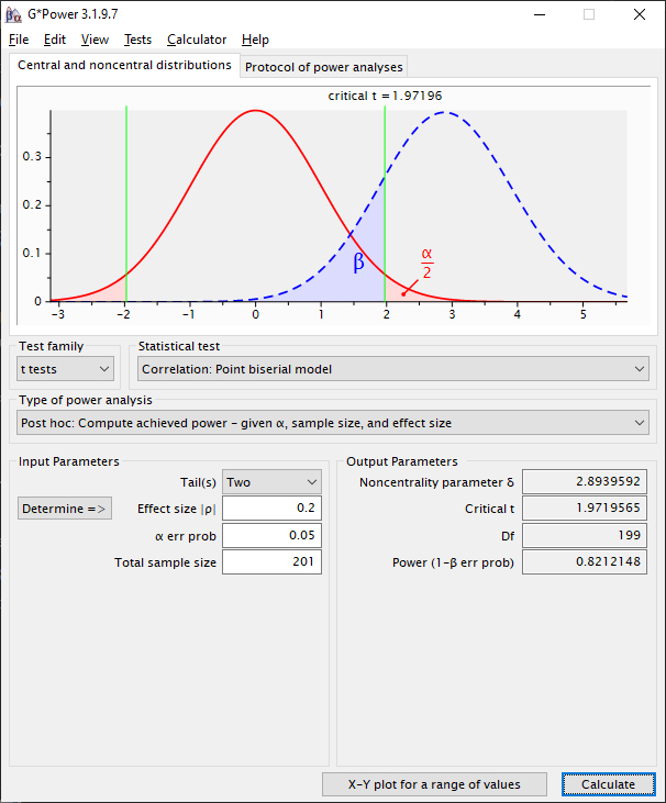
N = 100, k = 3, and rrm = 0.20. This design has 82% power.
install.packages("pwr")
require(pwr)

power.rmcorr <- function(k, N, effectsizer, sig)
    {pwr.r.test(n = ((N)*(k-1))+1, r = effectsizer, sig.level = sig)}

power.rmcorr(k = 3, N = 100, effectsizer = 0.20, sig = 0.05)
#>
#>      approximate correlation power calculation (arctangh transformation)
#>
#>               n = 201
#>               r = 0.2
#>       sig.level = 0.05
#>           power = 0.8156984
#>     alternative = two.sided
See Power curves for more information.
For G*Power (Faul et al. 2009) or other
software, power can be calculated by substituting the rmcorr degrees of
freedom for a Pearson correlation. Instead of sample size, use the
degrees of freedom for rmcorr plus two (effective sample size). This is
because a Pearson correlation has N - 2 degrees of
freedom.
- Rmcorr exact degrees of freedom = N x (k - 1) - 1
- Approximate degrees of freedom = (N -1) x (k - 1)
Exact Degrees of Freedom Example
Values: N = 100, k = 3 , and
rrm = 0.20 (same as above)
rmcorr df =
100 x (3 - 1) - 1 = 200 - 1 = 199
Add two (kludge): 199 + 2 = 201
Enter N = 201 as the effective sample size in G*Power
G*Power will calculate the degrees of freedom as N - 2 = 201 -
2 = 199. Thus, using the correct degrees of freedom for rmcorr.
Note power is just slighty different than the same calculation in R, which uses an arctan approximation.

Approximate Degrees of Freedom Example
Values: N = 100, k = 3, and
rrm = 0.20 (again, same as above)
approx rmcorr df = (100 - 1) x (3 - 1) = 99 x 2 = 198
Note the
small difference between the approximate vs. exact calculation:
one degree of freedom
Add two (same kludge) for G*Power,
entering a sample size of N = 200
Note power is slighty different than the exact formula
above. 
How to Extract the Slope and its Confidence Interval
my.rmc <- rmcorr(participant = Subject, measure1 = PaCO2, measure2 = pH,
                 dataset = bland1995)
#> Warning in rmcorr(participant = Subject, measure1 = PaCO2, measure2 = pH, :
#> 'Subject' coerced into a factor

# Structure of rmcorr object
#str(my.rmc)

# Extract rmcorr model coefficients
coef.rmc  <- my.rmc$model$coefficients
coef.rmc
#>  (Intercept) Participant1 Participant2 Participant3 Participant4 Participant5
#>   7.65590848  -0.72605418  -0.02144291   0.22395850   0.24550355   0.13432752
#> Participant6 Participant7     Measure1
#>   0.20037424  -0.03394863  -0.10832305

slope.rmc <- coef.rmc[length(coef.rmc)] #Last value in coefficients is the slope
slope.rmc
#>  Measure1
#> -0.108323

# Confidence intervals around all estimates
coef.CIs <- stats::confint(my.rmc$model)
coefs.all <- cbind(coef.rmc, coef.CIs)
coefs.all
#>                 coef.rmc       2.5 %      97.5 %
#> (Intercept)   7.65590848  7.34994594  7.96187102
#> Participant1 -0.72605418 -0.83211999 -0.61998837
#> Participant2 -0.02144291 -0.11116705  0.06828123
#> Participant3  0.22395850  0.16049969  0.28741732
#> Participant4  0.24550355  0.16448903  0.32651806
#> Participant5  0.13432752  0.05868538  0.20996967
#> Participant6  0.20037424  0.12673292  0.27401556
#> Participant7 -0.03394863 -0.17148111  0.10358385
#> Measure1     -0.10832305 -0.16883787 -0.04780822
isa Error
We have had reports of this error when running rmcorr:
Error in isa(Participant, "character") : could not find function "isa" Updating R to version 4.1.0 or later resolves this error.
Transformations
Transformations can be used to make the data (errors) more normal. We highly recommend graphing both the raw and transformed data. It may be appropriate to only transform one measure or transform both measures. “Consider transforming every variable in sight” (Gelman and Hill 2007, 548).
Limitations
Change Over Time
In general, rmcorr is a time-independent model– it does not model
change over time. A partial exception is if time is a measure, such as
age in the raz2005 dataset.
Non-Linearity
Rmcorr fits a linear model. If the data are non-linear, we recommend trying to transform it (see above) or using multilevel modeling. Also see Diagnostic Plots
Varying Slopes with Influential Observations and/or Unbalanced Data
If slopes meaningfully vary by individual, we recommend using
multilevel modeling instead of rmcorr. Random effect slopes are even
more problematic for rmcorr with influential observations and/or highly
unbalanced data. This is nicely illustrated in simulations by Dr. Marta
Karas:
When
rmcorr may not be ideal
Other Implementations of rmcorr
We know of three other implementations of rmcorr.